
Unraveling the Digital Brain: A Deep Dive into How Do Neural Networks Work
Affiliate disclosure: This article may contain affiliate links. Recommendations are independent and editorially driven.
In the rapidly accelerating landscape of artificial intelligence, few concepts are as foundational, yet as frequently misunderstood, as neural networks. These computational models, inspired by the intricate biological structures of the human brain, stand at the very core of modern AI breakthroughs, powering everything from sophisticated language models and lifelike image generation to autonomous vehicles and groundbreaking scientific discovery. Understanding how do neural networks work isn’t merely an academic exercise; it’s a critical lens through which to view the future of technology, automation, and even humanity itself.
For decades, the idea of machines thinking or learning remained largely within the realm of science fiction. Today, thanks to significant advancements in computational power, vast datasets, and innovative algorithms, neural networks have transcended theoretical discussions to become the engine driving the AI revolution. They are the digital architects behind the intelligence we increasingly encounter in our daily lives, often operating silently in the background, transforming industries, and redefining possibilities. But what are these complex systems, and how do they manage to extract patterns, learn from experience, and make decisions with astonishing accuracy?
This comprehensive guide from futureinsights aims to demystify neural networks, peeling back the layers of complexity to reveal their elegant underlying principles. We will embark on a journey from their biological inspirations to their fundamental components, delve into the intricate learning processes that enable them to adapt, explore the diverse architectures tailored for specific tasks, and ultimately, cast an eye towards their profound implications for our future. Whether you’re an aspiring AI enthusiast, a seasoned technologist, or simply curious about the forces shaping 2026 and beyond, grasping the mechanics of neural networks is paramount to navigating the evolving digital frontier.
The Biological Inspiration: A Glimpse into the Human Brain
Before we dissect the artificial constructs, it’s essential to appreciate the profound inspiration behind them: the human brain. Nature, through billions of years of evolution, has engineered the most sophisticated learning machine known. Our brains, teeming with billions of interconnected neurons, are the ultimate proof-of-concept for parallel processing, pattern recognition, and adaptive learning. The early pioneers of artificial intelligence sought to mimic this biological marvel, laying the groundwork for what we now call neural networks.
Neurons as Fundamental Building Blocks
At the heart of the brain’s incredible capabilities are individual cells called neurons. Each neuron is a complex processor, receiving signals from thousands of other neurons, integrating these signals, and, if the combined input is strong enough, generating its own signal to transmit to yet other neurons. This fundamental ‘on-or-off’ decision, based on a threshold, is the simplest form of computation in the brain. Artificial neural networks abstract this concept, creating artificial “nodes” or “perceptrons” that emulate this basic input-processing-output mechanism.
Synapses and Signal Transmission
Neurons don’t just exist in isolation; they form an intricate web of connections. These connections are called synapses. When a neuron fires, it sends an electrochemical signal across a synapse to a neighboring neuron. The strength of this synaptic connection determines how much influence one neuron has on another. This strength isn’t fixed; it can be adjusted through experience, a phenomenon known as synaptic plasticity. This adjustment is crucial for learning and memory formation. In artificial neural networks, these synaptic strengths are represented by “weights,” numerical values that dictate the importance of an input connection.
Learning Through Connection Strength Adjustment
The remarkable ability of the brain to learn, adapt, and remember stems from its capacity to modify the strength and efficacy of its synaptic connections. When you learn a new skill, form a new memory, or even simply recognize a face, your brain is physically (or functionally) altering the connections between its neurons. Stronger connections facilitate better signal transmission, reinforcing certain pathways, while weaker connections diminish their influence. This principle of learning by adjusting connection strengths is the cornerstone of how artificial neural networks are trained. They iteratively adjust their internal weights in response to data, striving to improve their performance on a given task, much like our brains refine their neural pathways over time.
Core Components of an Artificial Neural Network

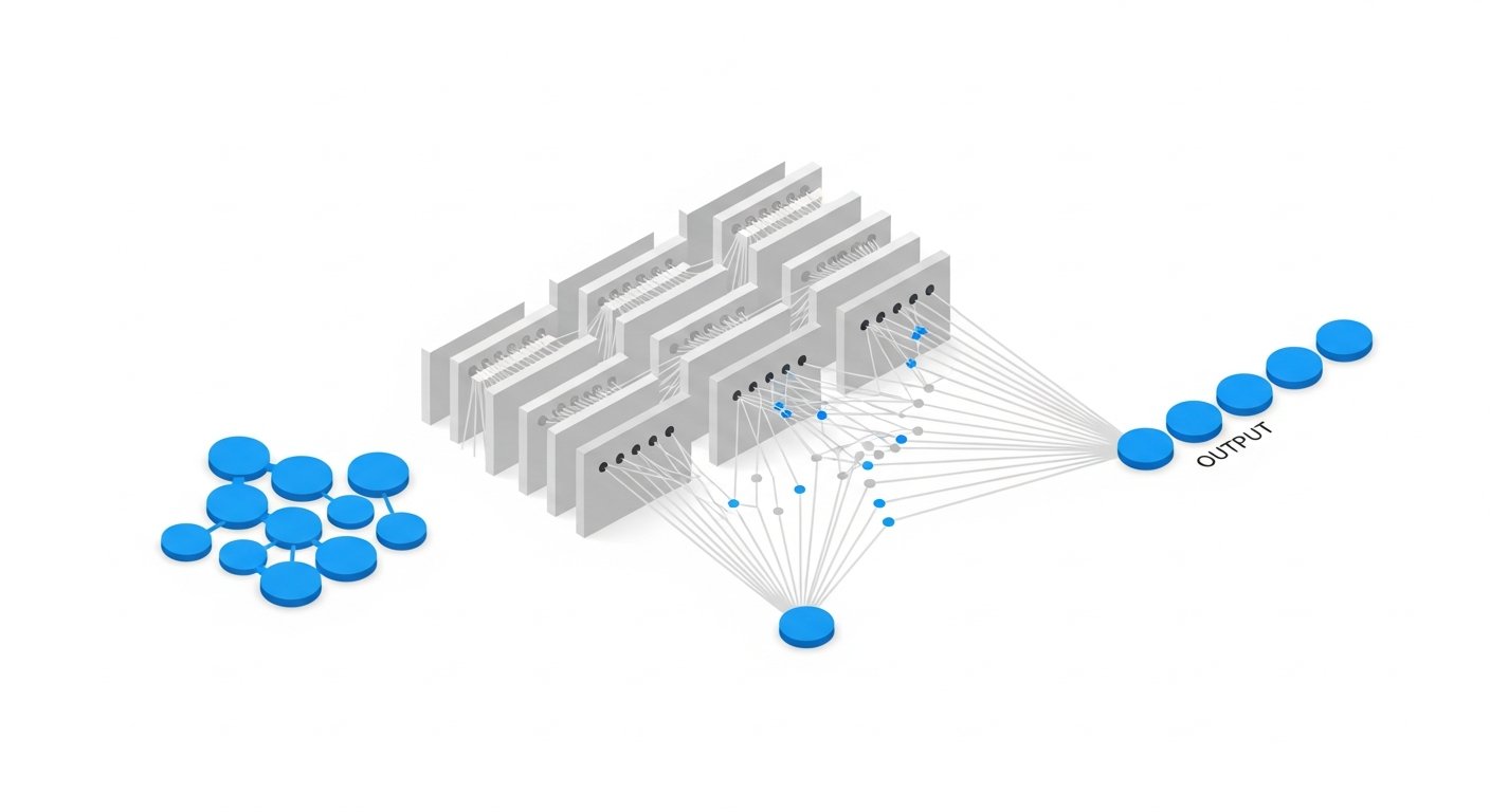
Having explored the biological blueprint, let’s transition to the digital realm. An artificial neural network (ANN) is not a physical entity but a computational model, a complex algorithm designed to recognize patterns and make predictions. Despite their often intimidating reputation, ANNs are built from relatively simple, interconnected components arranged in layers. Understanding these components is key to grasping how do neural networks work.
[INLINE IMAGE 1: place after second H2 | alt=”how do neural networks work concept illustration”]
Input Layer: Receiving the Data
Every neural network begins with an input layer. This layer is responsible for receiving the raw data that the network will process. Each “neuron” or node in the input layer corresponds to a specific feature or attribute of the input data. For example, if the network is designed to classify images, the input layer might consist of nodes representing individual pixels and their color values. If it’s analyzing financial data, the nodes might represent stock prices, trading volumes, or economic indicators. The input layer simply passes the data forward; it doesn’t perform any computations on its own.
Hidden Layers: The Engine of Abstraction
Between the input and output layers lie one or more hidden layers. These are the computational workhorses of the neural network. Each neuron in a hidden layer receives inputs from the neurons in the preceding layer, processes them, and then passes its output to the neurons in the subsequent layer. The “magic” of deep learning, a subfield of machine learning that heavily relies on neural networks, often comes from having multiple hidden layers. Each successive hidden layer learns to recognize increasingly complex and abstract patterns from the data. For instance, in image recognition, an early hidden layer might detect edges or simple shapes, while a deeper layer might combine these to recognize textures or parts of objects, and even deeper layers might identify entire objects like faces or cars. The ability to automatically learn hierarchical features without explicit programming is one of the most powerful aspects of neural networks.
Output Layer: Delivering the Prediction
The final layer of a neural network is the output layer. This layer is responsible for presenting the network’s final prediction or decision. The number of neurons in the output layer depends directly on the task the network is designed for. For a binary classification task (e.g., “yes” or “no,” “cat” or “dog”), there might be a single output neuron. For multi-class classification (e.g., identifying one of ten different digits), there would be one neuron for each class. For regression tasks (e.g., predicting a house price), there might be a single output neuron representing the continuous value. The values produced by the output layer are the network’s final answer after processing the input data through all its layers.
Neurons (Nodes) and Connections (Weights)
At its most fundamental level, a neural network is a collection of interconnected nodes, often visualized as circles. These nodes, or “neurons,” are organized into layers. Each connection between nodes carries a “weight,” which is a numerical value. This weight signifies the strength and importance of the connection, much like a biological synapse. A higher positive weight means that the input from that connection strongly contributes to activating the receiving neuron, while a negative weight might inhibit it. During the learning process, these weights are iteratively adjusted to improve the network’s performance. The collective adjustment of these weights across the entire network is how a neural network learns to map inputs to desired outputs.
Activation Functions: Introducing Non-Linearity
If neural networks only performed weighted sums of their inputs, they would essentially be limited to solving linear problems, severely restricting their utility. This is where activation functions come in. An activation function is a mathematical operation applied to the output of each neuron in the hidden and output layers. Its primary role is to introduce non-linearity into the network. Without non-linearity, no matter how many layers a network has, it would still behave like a single-layer network, unable to learn complex patterns. Common activation functions include the Sigmoid (squashing output between 0 and 1), Tanh (between -1 and 1), and the Rectified Linear Unit (ReLU), which outputs the input directly if positive, and zero otherwise. ReLU and its variants are particularly popular in deep learning due to their computational efficiency and ability to mitigate vanishing gradient problems.
Biases: Shifting the Activation Threshold
In addition to weights, each neuron (except those in the input layer) typically has an associated “bias” term. Think of a bias as an independent value that is added to the weighted sum of inputs before the activation function is applied. Its role is analogous to shifting the activation threshold of a biological neuron. A positive bias makes it easier for the neuron to activate, while a negative bias makes it harder. Biases allow the network to represent a wider range of functions and are crucial for the model’s flexibility. Without biases, the network would always have to pass through the origin (0,0) in its decision space, which severely limits its modeling capabilities. Together, weights and biases are the parameters that a neural network learns during its training phase.
The Learning Process: How Neural Networks Understand Data
The true power of neural networks lies not just in their architecture but in their ability to learn. Unlike traditional programming where rules are explicitly defined, neural networks learn from data, identifying underlying patterns and relationships. This learning process, often described as training, is what transforms a nascent network into a highly capable intelligent system. Understanding how do neural networks work fundamentally requires grasping this iterative learning cycle.
Forward Propagation: Making a Prediction
The learning process begins with forward propagation. In this phase, an input (e.g., an image, a sentence, a set of numerical features) is fed into the network’s input layer. This input then travels through the network, layer by layer, until it reaches the output layer. At each neuron, the inputs from the previous layer are multiplied by their respective weights, summed up, and then passed through an activation function. This processed output then becomes the input for the next layer. This sequential calculation from input to output generates the network’s initial prediction or output for the given input. Initially, with randomly initialized weights, this prediction will likely be inaccurate, but it’s the first step in the learning cycle.
Loss Functions: Quantifying Error
After the network makes a prediction through forward propagation, its performance needs to be evaluated. This is where a “loss function” (also known as a cost function or error function) comes into play. A loss function quantitatively measures the discrepancy between the network’s predicted output and the actual, correct target output (the “ground truth”). The larger the difference, the higher the loss. Different tasks require different loss functions. For example, in classification tasks, common loss functions include Cross-Entropy Loss, while for regression tasks, Mean Squared Error (MSE) is often used. The goal of training is to minimize this loss function, thereby making the network’s predictions as close as possible to the true values.
Backward Propagation (Backpropagation): The Learning Algorithm
Once the loss is calculated, the network needs a mechanism to adjust its weights and biases to reduce that error. This mechanism is called backpropagation (short for “backward propagation of errors”). Backpropagation is the cornerstone algorithm that enables neural networks to learn efficiently. It works by propagating the error backwards through the network, from the output layer towards the input layer. Using calculus (specifically, the chain rule for derivatives), backpropagation determines how much each individual weight and bias contributed to the overall error. It calculates the “gradient” of the loss function with respect to each parameter (weight and bias), indicating the direction and magnitude of adjustment needed for each parameter to decrease the loss.
Gradient Descent: Optimizing the Weights
With the gradients calculated by backpropagation, the network uses an optimization algorithm, most commonly “gradient descent,” to update its weights and biases. Imagine the loss function as a landscape with hills and valleys, and the goal is to find the lowest point (minimum loss). Gradient descent works by taking small steps in the direction opposite to the gradient (the steepest ascent). Each step, known as an iteration, slightly adjusts the weights and biases, bringing the network closer to a state where its predictions are more accurate. There are various flavors of gradient descent, such as Stochastic Gradient Descent (SGD), Mini-Batch Gradient Descent, and more advanced adaptive optimizers like Adam and RMSprop, which fine-tune how these steps are taken to accelerate convergence and avoid getting stuck in local minima.
Epochs, Batches, and Learning Rate
The entire learning process involves several key hyperparameters. An “epoch” refers to one complete pass of the entire training dataset through the neural network, both forward and backward. Since processing the entire dataset at once can be computationally intensive, data is often divided into “batches” or “mini-batches.” The network processes a batch, updates its weights, and then moves to the next batch. This batching strategy helps smooth out the learning process. The “learning rate” is another critical hyperparameter. It dictates the size of the steps taken during gradient descent. A high learning rate can lead to overshooting the minimum, while a very low learning rate can make training exceedingly slow. Finding the optimal learning rate is often a matter of experimentation and tuning, profoundly impacting how efficiently and effectively a neural network learns.
Explore advanced optimization techniques in AI training.
Types of Neural Networks and Their Applications
The foundational principles of neural networks – interconnected nodes, weighted connections, activation functions, and backpropagation – remain consistent across various architectures. However, the specific arrangement of these components, the nature of their connections, and the way they process information can vary significantly. This architectural diversity has given rise to specialized types of neural networks, each excelling at different tasks and solving distinct problems. Understanding these variations is crucial for appreciating the breadth of how do neural networks work in real-world applications.
[INLINE IMAGE 2: place after fourth H2 | alt=”how do neural networks work comparison illustration”]
Feedforward Neural Networks (FNNs)
The most basic and fundamental type of neural network is the Feedforward Neural Network (FNN), also known as a Multi-Layer Perceptron (MLP). In an FNN, information flows in only one direction: from the input layer, through any hidden layers, to the output layer. There are no loops or cycles in the network. Each neuron in a layer is connected to every neuron in the subsequent layer. FNNs are versatile and can be used for a wide range of tasks, including classification, regression, and pattern recognition in structured data. Despite their simplicity compared to more advanced architectures, they form the building blocks for understanding more complex networks and are still widely used for tasks where the input data is relatively independent across features.
Convolutional Neural Networks (CNNs): Vision’s Powerhouses
Convolutional Neural Networks (CNNs) have revolutionized computer vision, becoming the de-facto standard for tasks involving image and video processing. Unlike FNNs, CNNs leverage a specialized layer called a “convolutional layer,” which applies filters (small matrices of weights) across local regions of the input data. This process effectively extracts spatial hierarchies of features, such as edges, textures, and eventually complex objects, in an invariant manner (meaning it can detect features regardless of their exact position in the image). CNNs also often include “pooling layers” to downsample feature maps, reducing computational cost and making the network more robust to minor variations. Their success is evident in applications like facial recognition, medical image analysis, object detection in autonomous vehicles, and image generation.
Recurrent Neural Networks (RNNs): Handling Sequences
While FNNs and CNNs process inputs independently, Recurrent Neural Networks (RNNs) are specifically designed to handle sequential data, where the order of information matters. This makes them ideal for natural language processing (NLP), speech recognition, and time-series prediction. The key feature of an RNN is its “memory”: it maintains a hidden state that captures information about previous elements in the sequence. This hidden state is fed back into the network alongside the current input, allowing the network to make predictions that are contextually aware of past inputs. However, vanilla RNNs suffer from the “vanishing gradient problem,” making it difficult for them to learn long-term dependencies.
Long Short-Term Memory (LSTM) Networks: Addressing RNN Limitations
To overcome the vanishing gradient problem inherent in traditional RNNs, Long Short-Term Memory (LSTM) networks were developed. LSTMs are a special type of RNN that include sophisticated “gates” (input, forget, and output gates) within their memory cells. These gates control the flow of information, allowing LSTMs to selectively remember or forget past information over extended periods. This capability makes LSTMs incredibly effective at capturing long-range dependencies in sequential data. They have been instrumental in significant advancements in machine translation, speech-to-text conversion, sentiment analysis, and even generating coherent text and music.
Generative Adversarial Networks (GANs): The Creative Engine
Generative Adversarial Networks (GANs) represent a fascinating and powerful class of neural networks focused on generative tasks, meaning they can create new data instances that resemble the training data. A GAN consists of two competing neural networks: a “generator” and a “discriminator.” The generator’s role is to create realistic fake data (e.g., images of non-existent people), while the discriminator’s role is to distinguish between real data and the generator’s fakes. They are trained simultaneously in an adversarial game: the generator tries to fool the discriminator, and the discriminator tries to get better at catching fakes. This dynamic pushes both networks to improve, resulting in generators capable of producing incredibly convincing and novel outputs. GANs are behind applications like deepfakes, realistic image synthesis, style transfer, and data augmentation.
Transformers: Revolutionizing NLP
The Transformer architecture, introduced in 2017, has revolutionized Natural Language Processing (NLP) and is now making inroads into computer vision. Unlike RNNs and LSTMs, Transformers eschew recurrence and rely entirely on a mechanism called “self-attention.” Self-attention allows the network to weigh the importance of different words in an input sequence relative to each other, irrespective of their distance. This parallel processing capability addresses the sequential bottleneck of RNNs and LSTMs, enabling models to train on much longer sequences and much larger datasets. Transformers are the backbone of large language models (LLMs) like GPT-series, BERT, and countless others, powering advanced text generation, machine translation, summarization, and question-answering systems. Their ability to capture long-range dependencies and parallelize computation has made them one of the most impactful breakthroughs in AI of the past decade.
Comparison of Key Neural Network Architectures
To further illustrate the diverse capabilities and applications, here’s a comparative overview of some key neural network architectures:
| Architecture Type | Primary Strength | Typical Applications | Key Limitation / Challenge |
|---|---|---|---|
| Feedforward Neural Network (FNN / MLP) | Universal function approximation, good for structured data | Simple classification, regression, pattern recognition in tabular data | Lacks ability to process spatial or sequential dependencies efficiently; requires flattened inputs for images. |
| Convolutional Neural Network (CNN) | Excellent for spatial hierarchies, translation invariance | Image recognition, object detection, video analysis, medical imaging | Can be computationally intensive; sometimes struggles with rotational invariance without augmentation. |
| Recurrent Neural Network (RNN) | Processes sequential data, maintains “memory” of past inputs | Speech recognition, basic machine translation, time-series prediction | Suffers from vanishing/exploding gradient problems; difficulty learning long-term dependencies. |
| Long Short-Term Memory (LSTM) | Handles long-term dependencies in sequences, mitigates vanishing gradient | Advanced NLP (machine translation, sentiment analysis), complex time-series forecasting | More complex architecture than RNNs; slower to train due to sequential processing. |
| Generative Adversarial Network (GAN) | Generates realistic new data instances | Image synthesis, style transfer, data augmentation, deepfakes | Difficult to train (mode collapse, training instability); requires careful balancing of generator and discriminator. |
| Transformer Network | Excellent for long-range dependencies, parallelizable computation | Advanced NLP (LLMs, machine translation), increasingly in computer vision | Very high computational cost for long sequences (quadratic attention complexity); requires massive datasets. |
The choice of which neural network architecture to use depends heavily on the nature of the data and the specific problem to be solved. Often, hybrid architectures that combine elements of different types are employed for complex real-world challenges.
Training Strategies and Optimization Techniques
Building a neural network architecture is only half the battle; the other, equally critical half, is effectively training it. The raw computational power and vast datasets available today wouldn’t be nearly as impactful without sophisticated strategies and optimization techniques that allow neural networks to learn efficiently, avoid common pitfalls, and generalize well to unseen data. These methods are integral to understanding the practical realities of how do neural networks work in real-world deployments.
Data Preprocessing: The Foundation of Learning
The quality of the input data profoundly influences the performance of a neural network. Data preprocessing is a crucial initial step that involves cleaning, transforming, and preparing the raw data for consumption by the network. This can include:
- Normalization/Standardization: Scaling numerical features to a common range (e.g., 0-1 or mean 0, standard deviation 1) prevents features with larger values from dominating the learning process.
- Handling Missing Values: Imputing or removing missing data points.
- Encoding Categorical Data: Converting non-numerical categories (e.g., “red,” “green,” “blue”) into numerical representations (e.g., one-hot encoding).
- Feature Engineering: Creating new features from existing ones to potentially provide more relevant information to the network.
- Data Augmentation: Especially in image processing, generating new training examples by applying transformations (rotations, flips, zooms) to existing data, which helps improve generalization and reduce overfitting.
Proper data preprocessing reduces noise, speeds up training, and often leads to significantly better model performance.
Regularization: Preventing Overfitting
One of the most common challenges in training neural networks is “overfitting.” This occurs when a network learns the training data too well, memorizing noise and specific examples rather than generalizing underlying patterns. An overfit model performs exceptionally well on the training data but poorly on new, unseen data. Regularization techniques are designed to combat overfitting:
- L1 and L2 Regularization: These add a penalty term to the loss function based on the magnitude of the network’s weights. L1 (Lasso) encourages sparsity (some weights become zero), effectively performing feature selection. L2 (Ridge) encourages smaller weights overall.
- Dropout: During training, random subsets of neurons in a layer are temporarily “dropped out” (set to zero) along with their connections. This forces the network to learn more robust features and prevents neurons from co-adapting too much.
- Early Stopping: Monitoring the model’s performance on a separate validation dataset during training. When the validation error starts to increase (indicating overfitting), training is stopped.
These techniques help the network learn more generalizable representations, crucial for real-world reliability.
Hyperparameter Tuning: The Art of Configuration
Neural networks have numerous settings that are not learned from data but must be specified by the developer before training begins. These are called “hyperparameters.” Examples include the learning rate, the number of hidden layers, the number of neurons in each layer, the choice of activation functions, batch size, and the type of optimizer. Finding the optimal combination of hyperparameters is often more art than science and can significantly impact a network’s performance. Common tuning strategies include:
- Grid Search: Systematically trying every combination of hyperparameters from a predefined set.
- Random Search: Randomly sampling hyperparameter combinations, often more efficient than grid search for high-dimensional hyperparameter spaces.
- Bayesian Optimization: A more sophisticated approach that builds a probabilistic model of the objective function (e.g., validation loss) and uses it to select the most promising hyperparameters to evaluate next.
- Automated Machine Learning (AutoML): Emerging platforms that automate the entire hyperparameter tuning process, even exploring different architectures.
Effective hyperparameter tuning is essential for unlocking the full potential of a neural network.
Optimization Algorithms Beyond SGD (Adam, RMSprop)
While basic Stochastic Gradient Descent (SGD) forms the core of weight updates, more advanced optimization algorithms have been developed to accelerate and stabilize the training process, especially in deep neural networks. These optimizers often adapt the learning rate for each parameter individually or incorporate momentum to smooth out updates.
- Momentum: Helps accelerate SGD in the relevant direction and dampens oscillations by adding a fraction of the update vector from the past step to the current update.
- AdaGrad (Adaptive Gradient): Adapts the learning rate for each parameter, performing smaller updates for parameters associated with frequently occurring features and larger updates for rarely occurring features.
- RMSprop (Root Mean Square Propagation): Addresses AdaGrad’s diminishing learning rate issue by using a moving average of squared gradients.
- Adam (Adaptive Moment Estimation): Combines the concepts of RMSprop and momentum, maintaining an exponentially decaying average of past gradients and past squared gradients. Adam is widely considered one of the most effective and popular optimizers for deep learning.
The choice of optimizer can significantly impact training speed, convergence, and final model performance.
Learn more about the mathematics behind gradient descent.
Transfer Learning: Leveraging Pre-trained Models
Training a deep neural network from scratch, especially a complex one like a Transformer or a very deep CNN, requires immense computational resources and massive datasets. Transfer learning offers an elegant solution. It involves taking a pre-trained model – a neural network that has already been trained on a very large dataset for a similar task (e.g., an image classification model trained on millions of images) – and adapting it for a new, often smaller, dataset and a related task.
This is achieved by:
- Feature Extraction: Using the pre-trained model’s earlier layers as a fixed feature extractor and only training a new, smaller classification head (output layer) on top.
- Fine-tuning: Unfreezing some or all of the pre-trained layers and continuing training (with a very small learning rate) on the new dataset, allowing the model to adapt its learned features more specifically to the new task.
Transfer learning significantly reduces the computational burden and the amount of data required, making powerful neural network capabilities accessible even for problems with limited data. It’s a cornerstone of practical AI development in 2026.
Challenges and Limitations in Neural Network Development
While neural networks have undeniably propelled AI into an era of unprecedented capabilities, it’s equally important to acknowledge their inherent challenges and limitations. A holistic understanding of how do neural networks work must encompass not only their strengths but also the significant hurdles that researchers and developers face. Addressing these issues is critical for the responsible and effective deployment of AI systems in 2026 and beyond.
The Black Box Problem: Interpretability and Explainability (XAI)
Perhaps the most frequently cited limitation of deep neural networks is their “black box” nature. As networks grow in complexity, with billions of parameters across multiple hidden layers, it becomes incredibly difficult for humans to understand exactly why a particular decision or prediction was made. Unlike rule-based expert systems, neural networks learn abstract patterns that are not easily expressible as human-understandable logic. This lack of transparency, known as the interpretability problem, is a significant concern in critical applications such as:
- Medical Diagnosis: If an AI suggests a treatment, doctors need to understand the reasoning.
- Autonomous Vehicles: Why did the car make a specific maneuver?
- Financial Decisions: Justifying loan approvals or risk assessments.
The field of Explainable AI (XAI) is actively working to develop methods to provide insights into model decisions, such as attention mechanisms in Transformers or saliency maps in CNNs that highlight influential input regions, but it remains an active area of research.
Data Dependency and Bias
Neural networks are voracious consumers of data. Their performance is directly correlated with the quantity and quality of the training data. This dependence introduces several challenges:
- Data Scarcity: For niche applications or new domains, collecting enough labeled data can be prohibitively expensive or simply impossible.
- Data Quality: Noisy, incomplete, or incorrectly labeled data will lead to poor model performance, famously captured by the adage “garbage in, garbage out.”
- Bias Amplification: A more insidious problem is algorithmic bias. If the training data reflects existing societal biases (e.g., underrepresentation of certain demographic groups, historical prejudices), the neural network will learn and amplify these biases, leading to unfair or discriminatory outcomes. This has been observed in facial recognition systems, hiring algorithms, and even criminal justice tools. Mitigating bias requires careful data curation, bias detection techniques, and robust ethical frameworks.
Computational Cost and Resource Intensity
Training and deploying large, state-of-the-art neural networks demand immense computational resources.
- Hardware Requirements: Modern deep learning heavily relies on specialized hardware like Graphics Processing Units (GPUs) and Tensor Processing Units (TPUs), which are designed for parallel computations. Access to these resources can be expensive.
- Energy Consumption: Training a single large language model can consume energy equivalent to several trans-Atlantic flights or the lifetime carbon footprint of several cars. This raises significant environmental concerns, driving research into more energy-efficient architectures and training methods.
- Time Investment: Training complex models can take days, weeks, or even months, even with powerful hardware, limiting rapid iteration and experimentation.
The trend towards ever-larger models further exacerbates these resource constraints, creating a significant barrier to entry for smaller organizations and researchers.
Discover the latest advancements in energy-efficient AI.
Adversarial Attacks and Robustness Concerns
Despite their impressive performance, neural networks can be surprisingly vulnerable to subtle, maliciously crafted inputs known as “adversarial attacks.” These attacks involve making tiny, often imperceptible, perturbations to an input (e.g., an image) that cause the network to misclassify it with high confidence. For instance, a self-driving car’s vision system could be tricked into misinterpreting a stop sign as a yield sign by a few strategically placed pixels. This vulnerability raises serious security concerns for critical AI applications and highlights the need for developing more robust and resilient neural network models. Research into adversarial training and defense mechanisms is an urgent area of study.
Ethical Implications and Responsible AI
Beyond the technical challenges, the widespread adoption of powerful neural networks brings profound ethical implications.
- Job Displacement: Automation driven by AI, particularly through neural networks, could significantly disrupt labor markets, requiring societal adaptation and new economic models.
- Surveillance and Privacy: Advanced facial recognition, voice analysis, and behavior prediction capabilities raise concerns about mass surveillance and the erosion of individual privacy.
- Autonomous Decision-Making: As AI systems gain more autonomy, questions arise about accountability when mistakes occur, especially in life-or-death scenarios.
- Misinformation and Manipulation: Generative AI (like GANs and Transformers) can create highly realistic fake content (text, images, video), posing risks for misinformation campaigns, fraud, and psychological manipulation.
Developing and deploying AI responsibly requires not only technical solutions but also robust ethical guidelines, policy frameworks, and public discourse to ensure that these powerful technologies serve humanity’s best interests.
The Future Trajectory: What’s Next for Neural Networks?
The journey of neural networks has been one of continuous innovation, from theoretical concepts to practical, world-changing applications. As we look towards the mid-2020s and beyond, the trajectory of neural network development promises even more profound shifts, pushing the boundaries of what artificial intelligence can achieve and reshaping our understanding of intelligence itself. The question of how do neural networks work will evolve as new paradigms emerge.
Neuromorphic Computing: Hardware Inspired by Biology
Currently, most neural networks run on conventional silicon-based hardware (CPUs and GPUs) that operates fundamentally differently from the biological brain. The brain is massively parallel, event-driven, and highly energy-efficient. Neuromorphic computing aims to bridge this gap by developing specialized hardware architectures that directly mimic the brain’s structure and function. Instead of separate memory and processing units, neuromorphic chips integrate both, creating “spiking neural networks” where information is transmitted as discrete pulses (spikes), similar to biological neurons. This approach promises ultra-low power consumption and new levels of efficiency, which could be critical for deploying complex AI at the edge (e.g., in IoT devices, wearables, or autonomous drones) and unlocking capabilities for real-time, brain-like intelligence.
Quantum Neural Networks: A Paradigm Shift
Quantum computing, still in its nascent stages, holds the potential to revolutionize many computational fields, including AI. Quantum Neural Networks (QNNs) or quantum machine learning explore how quantum phenomena (such as superposition and entanglement) can be leveraged to build and train neural networks. While truly scalable quantum computers are still some years away, theoretical work and early experiments suggest that QNNs could offer exponential speedups for certain types of computations, potentially enabling neural networks to process vast amounts of data, learn complex patterns, and solve optimization problems that are currently intractable for classical computers. This could lead to breakthroughs in materials science, drug discovery, and cryptanalysis, fundamentally altering the landscape of AI capabilities.
Towards General Artificial Intelligence (AGI)
Current neural networks, despite their impressive capabilities, are largely “narrow AI” – highly proficient at specific tasks (e.g., playing chess, recognizing faces) but lacking generalized understanding or common sense. The long-term goal for many AI researchers is to achieve Artificial General Intelligence (AGI), systems that possess human-like cognitive abilities across a broad range of tasks, including reasoning, learning from limited data, creativity, and adaptability. While AGI remains a distant and complex challenge, advancements in neural network architectures (like the continually scaling Transformers), meta-learning (learning to learn), and self-supervised learning are bringing us closer. Future neural networks might feature more sophisticated cognitive architectures, integrate multiple modalities of information, and develop emergent properties that hint at generalized intelligence, though the path is fraught with philosophical and technical hurdles.
Read our in-depth analysis of the path to Artificial General Intelligence.
Autonomous AI Systems and Real-world Integration
{
“@context”: “https://schema.org”,
“@graph”: [
{
“@type”: “WebPage”,
“@id”: “https://www.futureinsights.com/how-do-neural-networks-work/”,
“url”: “https://www.futureinsights.com/how-do-neural-networks-work/”,
“name”: “How Do Neural Networks Work”,
“description”: “Article about how do neural networks work”,
“datePublished”: “2026-06-02”,
“dateModified”: “2026-06-02”,
“inLanguage”: “en-US”,
“isPartOf”: {
“@id”: “https://www.futureinsights.com/#website”
}
},
{
“@type”: “Article”,
“@id”: “https://www.futureinsights.com/how-do-neural-networks-work/#article”,
“headline”: “How Do Neural Networks Work”,
“name”: “How Do Neural Networks Work”,
“description”: “Article about how do neural networks work”,
“url”: “https://www.futureinsights.com/how-do-neural-networks-work/”,
“datePublished”: “2026-06-02”,
“dateModified”: “2026-06-02”,
“author”: {
“@type”: “Person”,
“@id”: “https://www.futureinsights.com/#author”,
“name”: “Editorial Team”
},
“publisher”: {
“@type”: “Organization”,
“@id”: “https://www.futureinsights.com/#organization”,
“name”: “Futureinsights”,
“url”: “https://www.futureinsights.com”
},
“mainEntityOfPage”: {
“@id”: “https://www.futureinsights.com/how-do-neural-networks-work/”
},
“keywords”: [
“how do neural networks work”
],
“articleSection”: “How Do Neural Networks Work”
},
{
“@type”: “BreadcrumbList”,
“@id”: “https://www.futureinsights.com/how-do-neural-networks-work/#breadcrumb”,
“itemListElement”: [
{
“@type”: “ListItem”,
“position”: 1,
“name”: “Home”,
“item”: “https://www.futureinsights.com”
},
{
“@type”: “ListItem”,
“position”: 2,
“name”: “How Do Neural Networks Work”,
“item”: “https://www.futureinsights.com/how-do-neural-networks-work/”
}
]
},
{
“@type”: “Organization”,
“@id”: “https://www.futureinsights.com/#organization”,
“name”: “Futureinsights”,
“url”: “https://www.futureinsights.com”
},
{
“@type”: “Person”,
“@id”: “https://www.futureinsights.com/#author”,
“name”: “Editorial Team”
}
]
}
Unraveling the Digital Brain: A Deep Dive into How Do Neural Networks Work
Affiliate disclosure: This article may contain affiliate links. Recommendations are independent and editorially driven.
In the rapidly accelerating landscape of artificial intelligence, few concepts are as foundational, yet as frequently misunderstood, as neural networks. These computational models, inspired by the intricate biological structures of the human brain, stand at the very core of modern AI breakthroughs, powering everything from sophisticated language models and lifelike image generation to autonomous vehicles and groundbreaking scientific discovery. Understanding how do neural networks work isn’t merely an academic exercise; it’s a critical lens through which to view the future of technology, automation, and even humanity itself.
For decades, the idea of machines thinking or learning remained largely within the realm of science fiction. Today, thanks to significant advancements in computational power, vast datasets, and innovative algorithms, neural networks have transcended theoretical discussions to become the engine driving the AI revolution. They are the digital architects behind the intelligence we increasingly encounter in our daily lives, often operating silently in the background, transforming industries, and redefining possibilities. But what are these complex systems, and how do they manage to extract patterns, learn from experience, and make decisions with astonishing accuracy?
This comprehensive guide from futureinsights aims to demystify neural networks, peeling back the layers of complexity to reveal their elegant underlying principles. We will embark on a journey from their biological inspirations to their fundamental components, delve into the intricate learning processes that enable them to adapt, explore the diverse architectures tailored for specific tasks, and ultimately, cast an eye towards their profound implications for our future. Whether you’re an aspiring AI enthusiast, a seasoned technologist, or simply curious about the forces shaping 2026 and beyond, grasping the mechanics of neural networks is paramount to navigating the evolving digital frontier.
The Biological Inspiration: A Glimpse into the Human Brain
Before we dissect the artificial constructs, it’s essential to appreciate the profound inspiration behind them: the human brain. Nature, through billions of years of evolution, has engineered the most sophisticated learning machine known. Our brains, teeming with billions of interconnected neurons, are the ultimate proof-of-concept for parallel processing, pattern recognition, and adaptive learning. The early pioneers of artificial intelligence sought to mimic this biological marvel, laying the groundwork for what we now call neural networks.
Neurons as Fundamental Building Blocks
At the heart of the brain’s incredible capabilities are individual cells called neurons. Each neuron is a complex processor, receiving signals from thousands of other neurons, integrating these signals, and, if the combined input is strong enough, generating its own signal to transmit to yet other neurons. This fundamental ‘on-or-off’ decision, based on a threshold, is the simplest form of computation in the brain. Artificial neural networks abstract this concept, creating artificial “nodes” or “perceptrons” that emulate this basic input-processing-output mechanism.
Synapses and Signal Transmission
Neurons don’t just exist in isolation; they form an intricate web of connections. These connections are called synapses. When a neuron fires, it sends an electrochemical signal across a synapse to a neighboring neuron. The strength of this synaptic connection determines how much influence one neuron has on another. This strength isn’t fixed; it can be adjusted through experience, a phenomenon known as synaptic plasticity. This adjustment is crucial for learning and memory formation. In artificial neural networks, these synaptic strengths are represented by “weights,” numerical values that dictate the importance of an input connection.
Learning Through Connection Strength Adjustment
The remarkable ability of the brain to learn, adapt, and remember stems from its capacity to modify the strength and efficacy of its synaptic connections. When you learn a new skill, form a new memory, or even simply recognize a face, your brain is physically (or functionally) altering the connections between its neurons. Stronger connections facilitate better signal transmission, reinforcing certain pathways, while weaker connections diminish their influence. This principle of learning by adjusting connection strengths is the cornerstone of how artificial neural networks are trained. They iteratively adjust their internal weights in response to data, striving to improve their performance on a given task, much like our brains refine their neural pathways over time.
Core Components of an Artificial Neural Network
Having explored the biological blueprint, let’s transition to the digital realm. An artificial neural network (ANN) is not a physical entity but a computational model, a complex algorithm designed to recognize patterns and make predictions. Despite their often intimidating reputation, ANNs are built from relatively simple, interconnected components arranged in layers. Understanding these components is key to grasping how do neural networks work.
[INLINE IMAGE 1: place after second H2 | alt=”how do neural networks work concept illustration”]
Input Layer: Receiving the Data
Every neural network begins with an input layer. This layer is responsible for receiving the raw data that the network will process. Each “neuron” or node in the input layer corresponds to a specific feature or attribute of the input data. For example, if the network is designed to classify images, the input layer might consist of nodes representing individual pixels and their color values. If it’s analyzing financial data, the nodes might represent stock prices, trading volumes, or economic indicators. The input layer simply passes the data forward; it doesn’t perform any computations on its own.
Hidden Layers: The Engine of Abstraction
Between the input and output layers lie one or more hidden layers. These are the computational workhorses of the neural network. Each neuron in a hidden layer receives inputs from the neurons in the preceding layer, processes them, and then passes its output to the neurons in the subsequent layer. The “magic” of deep learning, a subfield of machine learning that heavily relies on neural networks, often comes from having multiple hidden layers. Each successive hidden layer learns to recognize increasingly complex and abstract patterns from the data. For instance, in image recognition, an early hidden layer might detect edges or simple shapes, while a deeper layer might combine these to recognize textures or parts of objects, and even deeper layers might identify entire objects like faces or cars. The ability to automatically learn hierarchical features without explicit programming is one of the most powerful aspects of neural networks.
Output Layer: Delivering the Prediction
The final layer of a neural network is the output layer. This layer is responsible for presenting the network’s final prediction or decision. The number of neurons in the output layer depends directly on the task the network is designed for. For a binary classification task (e.g., “yes” or “no,” “cat” or “dog”), there might be a single output neuron. For multi-class classification (e.g., identifying one of ten different digits), there would be one neuron for each class. For regression tasks (e.g., predicting a house price), there might be a single output neuron representing the continuous value. The values produced by the output layer are the network’s final answer after processing the input data through all its layers.
Neurons (Nodes) and Connections (Weights)
At its most fundamental level, a neural network is a collection of interconnected nodes, often visualized as circles. These nodes, or “neurons,” are organized into layers. Each connection between nodes carries a “weight,” which is a numerical value. This weight signifies the strength and importance of the connection, much like a biological synapse. A higher positive weight means that the input from that connection strongly contributes to activating the receiving neuron, while a negative weight might inhibit it. During the learning process, these weights are iteratively adjusted to improve the network’s performance. The collective adjustment of these weights across the entire network is how a neural network learns to map inputs to desired outputs.
Activation Functions: Introducing Non-Linearity
If neural networks only performed weighted sums of their inputs, they would essentially be limited to solving linear problems, severely restricting their utility. This is where activation functions come in. An activation function is a mathematical operation applied to the output of each neuron in the hidden and output layers. Its primary role is to introduce non-linearity into the network. Without non-linearity, no matter how many layers a network has, it would still behave like a single-layer network, unable to learn complex patterns. Common activation functions include the Sigmoid (squashing output between 0 and 1), Tanh (between -1 and 1), and the Rectified Linear Unit (ReLU), which outputs the input directly if positive, and zero otherwise. ReLU and its variants are particularly popular in deep learning due to their computational efficiency and ability to mitigate vanishing gradient problems.
Biases: Shifting the Activation Threshold
In addition to weights, each neuron (except those in the input layer) typically has an associated “bias” term. Think of a bias as an independent value that is added to the weighted sum of inputs before the activation function is applied. Its role is analogous to shifting the activation threshold of a biological neuron. A positive bias makes it easier for the neuron to activate, while a negative bias makes it harder. Biases allow the network to represent a wider range of functions and are crucial for the model’s flexibility. Without biases, the network would always have to pass through the origin (0,0) in its decision space, which severely limits its modeling capabilities. Together, weights and biases are the parameters that a neural network learns during its training phase.
The Learning Process: How Neural Networks Understand Data
The true power of neural networks lies not just in their architecture but in their ability to learn. Unlike traditional programming where rules are explicitly defined, neural networks learn from data, identifying underlying patterns and relationships. This learning process, often described as training, is what transforms a nascent network into a highly capable intelligent system. Understanding how do neural networks work fundamentally requires grasping this iterative learning cycle.
Forward Propagation: Making a Prediction
The learning process begins with forward propagation. In this phase, an input (e.g., an image, a sentence, a set of numerical features) is fed into the network’s input layer. This input then travels through the network, layer by layer, until it reaches the output layer. At each neuron, the inputs from the previous layer are multiplied by their respective weights, summed up, and then passed through an activation function. This processed output then becomes the input for the next layer. This sequential calculation from input to output generates the network’s initial prediction or output for the given input. Initially, with randomly initialized weights, this prediction will likely be inaccurate, but it’s the first step in the learning cycle.
Loss Functions: Quantifying Error
After the network makes a prediction through forward propagation, its performance needs to be evaluated. This is where a “loss function” (also known as a cost function or error function) comes into play. A loss function quantitatively measures the discrepancy between the network’s predicted output and the actual, correct target output (the “ground truth”). The larger the difference, the higher the loss. Different tasks require different loss functions. For example, in classification tasks, common loss functions include Cross-Entropy Loss, while for regression tasks, Mean Squared Error (MSE) is often used. The goal of training is to minimize this loss function, thereby making the network’s predictions as close as possible to the true values.
Backward Propagation (Backpropagation): The Learning Algorithm
Once the loss is calculated, the network needs a mechanism to adjust its weights and biases to reduce that error. This mechanism is called backpropagation (short for “backward propagation of errors”). Backpropagation is the cornerstone algorithm that enables neural networks to learn efficiently. It works by propagating the error backwards through the network, from the output layer towards the input layer. Using calculus (specifically, the chain rule for derivatives), backpropagation determines how much each individual weight and bias contributed to the overall error. It calculates the “gradient” of the loss function with respect to each parameter (weight and bias), indicating the direction and magnitude of adjustment needed for each parameter to decrease the loss.
Gradient Descent: Optimizing the Weights
With the gradients calculated by backpropagation, the network uses an optimization algorithm, most commonly “gradient descent,” to update its weights and biases. Imagine the loss function as a landscape with hills and valleys, and the goal is to find the lowest point (minimum loss). Gradient descent works by taking small steps in the direction opposite to the gradient (the steepest ascent). Each step, known as an iteration, slightly adjusts the weights and biases, bringing the network closer to a state where its predictions are more accurate. There are various flavors of gradient descent, such as Stochastic Gradient Descent (SGD), Mini-Batch Gradient Descent, and more advanced adaptive optimizers like Adam and RMSprop, which fine-tune how these steps are taken to accelerate convergence and avoid getting stuck in local minima.
Epochs, Batches, and Learning Rate
The entire learning process involves several key hyperparameters. An “epoch” refers to one complete pass of the entire training dataset through the neural network, both forward and backward. Since processing the entire dataset at once can be computationally intensive, data is often divided into “batches” or “mini-batches.” The network processes a batch, updates its weights, and then moves to the next batch. This batching strategy helps smooth out the learning process. The “learning rate” is another critical hyperparameter. It dictates the size of the steps taken during gradient descent. A high learning rate can lead to overshooting the minimum, while a very low learning rate can make training exceedingly slow. Finding the optimal learning rate is often a matter of experimentation and tuning, profoundly impacting how efficiently and effectively a neural network learns.
Explore advanced optimization techniques in AI training.
Types of Neural Networks and Their Applications
The foundational principles of neural networks – interconnected nodes, weighted connections, activation functions, and backpropagation – remain consistent across various architectures. However, the specific arrangement of these components, the nature of their connections, and the way they process information can vary significantly. This architectural diversity has given rise to specialized types of neural networks, each excelling at different tasks and solving distinct problems. Understanding these variations is crucial for appreciating the breadth of how do neural networks work in real-world applications.
[INLINE IMAGE 2: place after fourth H2 | alt=”how do neural networks work comparison illustration”]
Feedforward Neural Networks (FNNs)
The most basic and fundamental type of neural network is the Feedforward Neural Network (FNN), also known as a Multi-Layer Perceptron (MLP). In an FNN, information flows in only one direction: from the input layer, through any hidden layers, to the output layer. There are no loops or cycles in the network. Each neuron in a layer is connected to every neuron in the subsequent layer. FNNs are versatile and can be used for a wide range of tasks, including classification, regression, and pattern recognition in structured data. Despite their simplicity compared to more advanced architectures, they form the building blocks for understanding more complex networks and are still widely used for tasks where the input data is relatively independent across features.
Convolutional Neural Networks (CNNs): Vision’s Powerhouses
Convolutional Neural Networks (CNNs) have revolutionized computer vision, becoming the de-facto standard for tasks involving image and video processing. Unlike FNNs, CNNs leverage a specialized layer called a “convolutional layer,” which applies filters (small matrices of weights) across local regions of the input data. This process effectively extracts spatial hierarchies of features, such as edges, textures, and eventually complex objects, in an invariant manner (meaning it can detect features regardless of their exact position in the image). CNNs also often include “pooling layers” to downsample feature maps, reducing computational cost and making the network more robust to minor variations. Their success is evident in applications like facial recognition, medical image analysis, object detection in autonomous vehicles, and image generation.
Recurrent Neural Networks (RNNs): Handling Sequences
While FNNs and CNNs process inputs independently, Recurrent Neural Networks (RNNs) are specifically designed to handle sequential data, where the order of information matters. This makes them ideal for natural language processing (NLP), speech recognition, and time-series prediction. The key feature of an RNN is its “memory”: it maintains a hidden state that captures information about previous elements in the sequence. This hidden state is fed back into the network alongside the current input, allowing the network to make predictions that are contextually aware of past inputs. However, vanilla RNNs suffer from the “vanishing gradient problem,” making it difficult for them to learn long-term dependencies.
Long Short-Term Memory (LSTM) Networks: Addressing RNN Limitations
To overcome the vanishing gradient problem inherent in traditional RNNs, Long Short-Term Memory (LSTM) networks were developed. LSTMs are a special type of RNN that include sophisticated “gates” (input, forget, and output gates) within their memory cells. These gates control the flow of information, allowing LSTMs to selectively remember or forget past information over extended periods. This capability makes LSTMs incredibly effective at capturing long-range dependencies in sequential data. They have been instrumental in significant advancements in machine translation, speech-to-text conversion, sentiment analysis, and even generating coherent text and music.
Generative Adversarial Networks (GANs): The Creative Engine
Generative Adversarial Networks (GANs) represent a fascinating and powerful class of neural networks focused on generative tasks, meaning they can create new data instances that resemble the training data. A GAN consists of two competing neural networks: a “generator” and a “discriminator.” The generator’s role is to create realistic fake data (e.g., images of non-existent people), while the discriminator’s role is to distinguish between real data and the generator’s fakes. They are trained simultaneously in an adversarial game: the generator tries to fool the discriminator, and the discriminator tries to get better at catching fakes. This dynamic pushes both networks to improve, resulting in generators capable of producing incredibly convincing and novel outputs. GANs are behind applications like deepfakes, realistic image synthesis, style transfer, and data augmentation.
Transformers: Revolutionizing NLP
The Transformer architecture, introduced in 2017, has revolutionized Natural Language Processing (NLP) and is now making inroads into computer vision. Unlike RNNs and LSTMs, Transformers eschew recurrence and rely entirely on a mechanism called “self-attention.” Self-attention allows the network to weigh the importance of different words in an input sequence relative to each other, irrespective of their distance. This parallel processing capability addresses the sequential bottleneck of RNNs and LSTMs, enabling models to train on much longer sequences and much larger datasets. Transformers are the backbone of large language models (LLMs) like GPT-series, BERT, and countless others, powering advanced text generation, machine translation, summarization, and question-answering systems. Their ability to capture long-range dependencies and parallelize computation has made them one of the most impactful breakthroughs in AI of the past decade.
Comparison of Key Neural Network Architectures
To further illustrate the diverse capabilities and applications, here’s a comparative overview of some key neural network architectures:
| Architecture Type | Primary Strength | Typical Applications | Key Limitation / Challenge |
|---|---|---|---|
| Feedforward Neural Network (FNN / MLP) | Universal function approximation, good for structured data | Simple classification, regression, pattern recognition in tabular data | Lacks ability to process spatial or sequential dependencies efficiently; requires flattened inputs for images. |
| Convolutional Neural Network (CNN) | Excellent for spatial hierarchies, translation invariance | Image recognition, object detection, video analysis, medical imaging | Can be computationally intensive; sometimes struggles with rotational invariance without augmentation. |
| Recurrent Neural Network (RNN) | Processes sequential data, maintains “memory” of past inputs | Speech recognition, basic machine translation, time-series prediction | Suffers from vanishing/exploding gradient problems; difficulty learning long-term dependencies. |
| Long Short-Term Memory (LSTM) | Handles long-term dependencies in sequences, mitigates vanishing gradient | Advanced NLP (machine translation, sentiment analysis), complex time-series forecasting | More complex architecture than RNNs; slower to train due to sequential processing. |
| Generative Adversarial Network (GAN) | Generates realistic new data instances | Image synthesis, style transfer, data augmentation, deepfakes | Difficult to train (mode collapse, training instability); requires careful balancing of generator and discriminator. |
| Transformer Network | Excellent for long-range dependencies, parallelizable computation | Advanced NLP (LLMs, machine translation), increasingly in computer vision | Very high computational cost for long sequences (quadratic attention complexity); requires massive datasets. |
The choice of which neural network architecture to use depends heavily on the nature of the data and the specific problem to be solved. Often, hybrid architectures that combine elements of different types are employed for complex real-world challenges.
Training Strategies and Optimization Techniques
Building a neural network architecture is only half the battle; the other, equally critical half, is effectively training it. The raw computational power and vast datasets available today wouldn’t be nearly as impactful without sophisticated strategies and optimization techniques that allow neural networks to learn efficiently, avoid common pitfalls, and generalize well to unseen data. These methods are integral to understanding the practical realities of how do neural networks work in real-world deployments.
Data Preprocessing: The Foundation of Learning
The quality of the input data profoundly influences the performance of a neural network. Data preprocessing is a crucial initial step that involves cleaning, transforming, and preparing the raw data for consumption by the network. This can include:
- Normalization/Standardization: Scaling numerical features to a common range (e.g., 0-1 or mean 0, standard deviation 1) prevents features with larger values from dominating the learning process.
- Handling Missing Values: Imputing or removing missing data points.
- Encoding Categorical Data: Converting non-numerical categories (e.g., “red,” “green,” “blue”) into numerical representations (e.g., one-hot encoding).
- Feature Engineering: Creating new features from existing ones to potentially provide more relevant information to the network.
- Data Augmentation: Especially in image processing, generating new training examples by applying transformations (rotations, flips, zooms) to existing data, which helps improve generalization and reduce overfitting.
Proper data preprocessing reduces noise, speeds up training, and often leads to significantly better model performance.
Regularization: Preventing Overfitting
One of the most common challenges in training neural networks is “overfitting.” This occurs when a network learns the training data too well, memorizing noise and specific examples rather than generalizing underlying patterns. An overfit model performs exceptionally well on the training data but poorly on new, unseen data. Regularization techniques are designed to combat overfitting:
- L1 and L2 Regularization: These add a penalty term to the loss function based on the magnitude of the network’s weights. L1 (Lasso) encourages sparsity (some weights become zero), effectively performing feature selection. L2 (Ridge) encourages smaller weights overall.
- Dropout: During training, random subsets of neurons in a layer are temporarily “dropped out” (set to zero) along with their connections. This forces the network to learn more robust features and prevents neurons from co-adapting too much.
- Early Stopping: Monitoring the model’s performance on a separate validation dataset during training. When the validation error starts to increase (indicating overfitting), training is stopped.
These techniques help the network learn more generalizable representations, crucial for real-world reliability.
Hyperparameter Tuning: The Art of Configuration
Neural networks have numerous settings that are not learned from data but must be specified by the developer before training begins. These are called “hyperparameters.” Examples include the learning rate, the number of hidden layers, the number of neurons in each layer, the choice of activation functions, batch size, and the type of optimizer. Finding the optimal combination of hyperparameters is often more art than science and can significantly impact a network’s performance. Common tuning strategies include:
- Grid Search: Systematically trying every combination of hyperparameters from a predefined set.
- Random Search: Randomly sampling hyperparameter combinations, often more efficient than grid search for high-dimensional hyperparameter spaces.
- Bayesian Optimization: A more sophisticated approach that builds a probabilistic model of the objective function (e.g., validation loss) and uses it to select the most promising hyperparameters to evaluate next.
- Automated Machine Learning (AutoML): Emerging platforms that automate the entire hyperparameter tuning process, even exploring different architectures.
Effective hyperparameter tuning is essential for unlocking the full potential of a neural network.
Optimization Algorithms Beyond SGD (Adam, RMSprop)
While basic Stochastic Gradient Descent (SGD) forms the core of weight updates, more advanced optimization algorithms have been developed to accelerate and stabilize the training process, especially in deep neural networks. These optimizers often adapt the learning rate for each parameter individually or incorporate momentum to smooth out updates.
- Momentum: Helps accelerate SGD in the relevant direction and dampens oscillations by adding a fraction of the update vector from the past step to the current update.
- AdaGrad (Adaptive Gradient): Adapts the learning rate for each parameter, performing smaller updates for parameters associated with frequently occurring features and larger updates for rarely occurring features.
- RMSprop (Root Mean Square Propagation): Addresses AdaGrad’s diminishing learning rate issue by using a moving average of squared gradients.
- Adam (Adaptive Moment Estimation): Combines the concepts of RMSprop and momentum, maintaining an exponentially decaying average of past gradients and past squared gradients. Adam is widely considered one of the most effective and popular optimizers for deep learning.
The choice of optimizer can significantly impact training speed, convergence, and final model performance.
Learn more about the mathematics behind gradient descent.
Transfer Learning: Leveraging Pre-trained Models
Training a deep neural network from scratch, especially a complex one like a Transformer or a very deep CNN, requires immense computational resources and massive datasets. Transfer learning offers an elegant solution. It involves taking a pre-trained model – a neural network that has already been trained on a very large dataset for a similar task (e.g., an image classification model trained on millions of images) – and adapting it for a new, often smaller, dataset and a related task.
This is achieved by:
- Feature Extraction: Using the pre-trained model’s earlier layers as a fixed feature extractor and only training a new, smaller classification head (output layer) on top.
- Fine-tuning: Unfreezing some or all of the pre-trained layers and continuing training (with a very small learning rate) on the new dataset, allowing the model to adapt its learned features more specifically to the new task.
Transfer learning significantly reduces the computational burden and the amount of data required, making powerful neural network capabilities accessible even for problems with limited data. It’s a cornerstone of practical AI development in 2026.
Challenges and Limitations in Neural Network Development
While neural networks have undeniably propelled AI into an era of unprecedented capabilities, it’s equally important to acknowledge their inherent challenges and limitations. A holistic understanding of how do neural networks work must encompass not only their strengths but also the significant hurdles that researchers and developers face. Addressing these issues is critical for the responsible and effective deployment of AI systems in 2026 and beyond.
The Black Box Problem: Interpretability and Explainability (XAI)
Perhaps the most frequently cited limitation of deep neural networks is their “black box” nature. As networks grow in complexity, with billions of parameters across multiple hidden layers, it becomes incredibly difficult for humans to understand exactly why a particular decision or prediction was made. Unlike rule-based expert systems, neural networks learn abstract patterns that are not easily expressible as human-understandable logic. This lack of transparency, known as the interpretability problem, is a significant concern in critical applications such as:
- Medical Diagnosis: If an AI suggests a treatment, doctors need to understand the reasoning.
- Autonomous Vehicles: Why did the car make a specific maneuver?
- Financial Decisions: Justifying loan approvals or risk assessments.
The field of Explainable AI (XAI) is actively working to develop methods to provide insights into model decisions, such as attention mechanisms in Transformers or saliency maps in CNNs that highlight influential input regions, but it remains an active area of research.
Data Dependency and Bias
Neural networks are voracious consumers of data. Their performance is directly correlated with the quantity and quality of the training data. This dependence introduces several challenges:
- Data Scarcity: For niche applications or new domains, collecting enough labeled data can be prohibitively expensive or simply impossible.
- Data Quality: Noisy, incomplete, or incorrectly labeled data will lead to poor model performance, famously captured by the adage “garbage in, garbage out.”
- Bias Amplification: A more insidious problem is algorithmic bias. If the training data reflects existing societal biases (e.g., underrepresentation of certain demographic groups, historical prejudices), the neural network will learn and amplify these biases, leading to unfair or discriminatory outcomes. This has been observed in facial recognition systems, hiring algorithms, and even criminal justice tools. Mitigating bias requires careful data curation, bias detection techniques, and robust ethical frameworks.
Computational Cost and Resource Intensity
Training and deploying large, state-of-the-art neural networks demand immense computational resources.
- Hardware Requirements: Modern deep learning heavily relies on specialized hardware like Graphics Processing Units (GPUs) and Tensor Processing Units (TPUs), which are designed for parallel computations. Access to these resources can be expensive.
- Energy Consumption: Training a single large language model can consume energy equivalent to several trans-Atlantic flights or the lifetime carbon footprint of several cars. This raises significant environmental concerns, driving research into more energy-efficient architectures and training methods.
- Time Investment: Training complex models can take days, weeks, or even months, even with powerful hardware, limiting rapid iteration and experimentation.
The trend towards ever-larger models further exacerbates these resource constraints, creating a significant barrier to entry for smaller organizations and researchers.
Discover the latest advancements in energy-efficient AI.
Adversarial Attacks and Robustness Concerns
Despite their impressive performance, neural networks can be surprisingly vulnerable to subtle, maliciously crafted inputs known as “adversarial attacks.” These attacks involve making tiny, often imperceptible, perturbations to an input (e.g., an image) that cause the network to misclassify it with high confidence. For instance, a self-driving car’s vision system could be tricked into misinterpreting a stop sign as a yield sign by a few strategically placed pixels. This vulnerability raises serious security concerns for critical AI applications and highlights the need for developing more robust and resilient neural network models. Research into adversarial training and defense mechanisms is an urgent area of study.
Ethical Implications and Responsible AI
Beyond the technical challenges, the widespread adoption of powerful neural networks brings profound ethical implications.
- Job Displacement: Automation driven by AI, particularly through neural networks, could significantly disrupt labor markets, requiring societal adaptation and new economic models.
- Surveillance and Privacy: Advanced facial recognition, voice analysis, and behavior prediction capabilities raise concerns about mass surveillance and the erosion of individual privacy.
- Autonomous Decision-Making: As AI systems gain more autonomy, questions arise about accountability when mistakes occur, especially in life-or-death scenarios.
- Misinformation and Manipulation: Generative AI (like GANs and Transformers) can create highly realistic fake content (text, images, video), posing risks for misinformation campaigns, fraud, and psychological manipulation.
Developing and deploying AI responsibly requires not only technical solutions but also robust ethical guidelines, policy frameworks, and public discourse to ensure that these powerful technologies serve humanity’s best interests.
The Future Trajectory: What’s Next for Neural Networks?
The journey of neural networks has been one of continuous innovation, from theoretical concepts to practical, world-changing applications. As we look towards the mid-2020s and beyond, the trajectory of neural network development promises even more profound shifts, pushing the boundaries of what artificial intelligence can achieve and reshaping our understanding of intelligence itself. The question of how do neural networks work will evolve as new paradigms emerge.
Neuromorphic Computing: Hardware Inspired by Biology
Currently, most neural networks run on conventional silicon-based hardware (CPUs and GPUs) that operates fundamentally differently from the biological brain. The brain is massively parallel, event-driven, and highly energy-efficient. Neuromorphic computing aims to bridge this gap by developing specialized hardware architectures that directly mimic the brain’s structure and function. Instead of separate memory and processing units, neuromorphic chips integrate both, creating “spiking neural networks” where information is transmitted as discrete pulses (spikes), similar to biological neurons. This approach promises ultra-low power consumption and new levels of efficiency, which could be critical for deploying complex AI at the edge (e.g., in IoT devices, wearables, or autonomous drones) and unlocking capabilities for real-time, brain-like intelligence.
Quantum Neural Networks: A Paradigm Shift
Quantum computing, still in its nascent stages, holds the potential to revolutionize many computational fields, including AI. Quantum Neural Networks (QNNs) or quantum machine learning explore how quantum phenomena (such as superposition and entanglement) can be leveraged to build and train neural networks. While truly scalable quantum computers are still some years away, theoretical work and early experiments suggest that QNNs could offer exponential speedups for certain types of computations, potentially enabling neural networks to process vast amounts of data, learn complex patterns, and solve optimization problems that are currently intractable for classical computers. This could lead to breakthroughs in materials science, drug discovery, and cryptanalysis, fundamentally altering the landscape of AI capabilities.
Towards General Artificial Intelligence (AGI)
Current neural networks, despite their impressive capabilities, are largely “narrow AI” – highly proficient at specific tasks (e.g., playing chess, recognizing faces) but lacking generalized understanding or common sense. The long-term goal for many AI researchers is to achieve Artificial General Intelligence (AGI), systems that possess human-like cognitive abilities across a broad range of tasks, including reasoning, learning from limited data, creativity, and adaptability. While AGI remains a distant and complex challenge, advancements in neural network architectures (like the continually scaling Transformers), meta-learning (learning to learn), and self-supervised learning are bringing us closer. Future neural networks might feature more sophisticated cognitive architectures, integrate multiple modalities of information, and develop emergent properties that hint at generalized intelligence, though the path is fraught with philosophical and technical hurdles.
Read our in-depth analysis of the path to Artificial General Intelligence.
Autonomous AI Systems and Real-world Integration
<p